6 Family of discrete random variables
In the following sections we will discuss some commonly used discrete probability distributions which are used to predict number of success in finite number of random trials, or number of occurrence in a given interval or space and so on.
6.1 Bernoulli distribution/r.v
Bernoulli r.v comes from Bernoulli trial-a trial which has TWO possible outcomes (success or failure).
Consider the toss of a biased coin, which comes up a head with probability \(p\), and a tail with probability \(1 - p\). The Bernoulli random variable takes the two values 1 and 0, depending on whether the outcome is a head or a tail:
\[
X=1 ; if \ \ a \ \ head,\\
X=0 ; if\ \ a \ \ tail.
\]
PMF: \(P(X=x)=f(x)=p^x (1-p)^{1-x}; \ \ x=0,1\)
Mean: \(E(X)=p\)
Variance: \(Var(X)=p(1-p)\)
For all its simplicity, the Bernoulli random variable is very important. In practice, it is used to model generic probabilistic situations with just two outcomes, such as:
(a) The state of a telephone at a given time that can be either free or busy.
(b) A person who can be either healthy or sick with a certain disease.
(c) The preference of a person who can be either for or against a certain political candidate.
Furthermore, by combining multiple Bernoulli random variables, one can construct more complicated random variables.
Note
Derivation of Mean and Variance of Bernoulli r.v
Mean:
\[E(X)=\sum_{x=0}^1 x\cdot f(x)=(0) f(0)+(1)f(1)=0+1\cdotp p=p\]
Variance:
\(Var(X)=E(X^2)-[E(X)]^2=p-p^2=p(1-p)\)
6.2 Binomial r.v
In a Binomial experiment , the Bernoulli trial is repeated \(n\) times with the following conditions:
a) The trials are independent
b) In each trial \(P(success)=p\) remains constant
Suppose \(X=number \ \ of \ \ successs \ \ in \ \ n\ \ trials\). Then \(X\) is called a Binomial r.v or follows Binomial distribution.
PMF: \[P(X=x)=f(x)=\binom {n}{x} p^x (1-p)^{n-x} ; x=0,1,2,...,n\]
Mean: \(E(X)=np\)
Variance: \(Var(X)=np(1-p)\)
We write \(X\sim Bin (n,p)\)
Note
If \(Y=number \ \ of \ \ failures\ \ in \ \ n\ \ trials\) then
\(Y\sim Bin(n,1-p)\)
Relation between Bernoulli r.v and Binomial r.v
A Binomial Random Variable Is a Sum of Bernoulli Random Variables
Let, \(Y_i\) is a Bernoulli r.v appeared in \(i^{th}\) Bernoulli trial. If we conduct \(n\) independent Bernoulli trials then we have \(n\) independent Bernoulli r.vs such as \(Y_1, Y_2, ..., Y_n\). Each \(Y_i\) has values of either \(1\) or \(0\).
Now if \(X\) is a Binomial r.v then,
\[ X=Y_1+Y_2+...+Y_n =\sum_{i=1}^n Y_i \]
Note
Derivation of Mean and Variance of Binomial r.v
From previous note, we know if \(Y_i\) is a Bernoulli r.v then
\(E(Y_i)=p\) and \(Var(Y_i)=p(1-p)\)
So, the mean of Binomial r.v that is
\[ E(X)=E(Y_1+Y_2+...+Y_n) \]
\[ =E(Y_1)+E(Y_2)+...+E(Y_n) \]
\[ =p+p+...+p=np \]
Now, the variance of \(X\) is:
\[ Var(X)=Var(Y_1+Y_2+...+Y_n) \]
\[ =Var(Y_1)+Var(Y_2)+...+Var(Y_n) \]
\[ =p(1-p)+p(1-p)+...+p(1-p)=np(1-p) \]
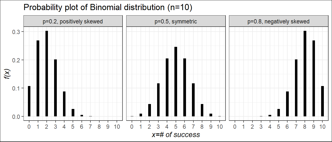
Probability plot of binomial r.v for different values of \(p\) and shape characteristics
Example 5.4 Consider a binomial experiment with \(n = 10\) and \(p =0.30\).
a) Compute \(P(X=0)\) ; b) Compute \(P(X=2)\);
c) Compute \(P(X \le 1)\) ; d) Compute \(P(X\ge 2)\);
e) Compute \(E(X)\) ; f) Compute \(Var(X)\) and \(\sigma\).
Example 5.5 A manufacturer of window frames knows from long experience that 30 percent of the production will have some type of minor defect that will require an adjustment. What is the probability that in a sample of 20 window frames:
a) none will need adjustment?
b) at most two will need adjustment?
c) at least two will need adjustment?
d) Estimate the mean and standard deviation of number of adjustment.
Example 5.6 A certain type of tomato seed germinates 90% of the time. A backyard farmer planted 25 seeds.
a) What is the probability that exactly 20 germinate?
b) What is the probability that 23 or more germinate?
c) What is the probability that 24 or fewer germinate?
d) What is the expected number of seeds that germinate?
Example 5.7 A shoe store’s records show that 30% of customers making a purchase use a credit card to pay. This morning, 10 customers purchased shoes from the store. Answer the following:
a) Find the probability that at least 8 of the customers used a credit card.
b) What is the probability that at least three customers, but not more than five, used a credit card?
c) What is the expected number of customers who used a credit card? What is the standard deviation?
*d) Find the probability that exactly 5 customers did not use a credit card.
*e) Find the probability that at least nine customers did not use a credit card
6.3 Poisson r.v
In this section we consider a discrete random variable that is often useful in estimating the number of occurrences over a specified interval of time or space. For example, the random variable of interest might be
the number of arrivals at a car wash in one hour,
the number of repairs needed in 10 miles of highway, or
the number of leaks in 100 miles of pipeline.
PROPERTIES OF A POISSON EXPERIMENT
The probability of an occurrence is the same for any two intervals of equal length.
The occurrence or nonoccurrence in any interval is independent of the occurrence or nonoccurrence in any other interval.
Suppose \(X\) be the number occurrences in a given interval. Then,
PMF:
\[ P(X=x)=f(x)=\frac{\mu^x e^{-\mu}}{x!}\ \ ; \ \ x=0,1,2,...,\infty \]
Where, \(\mu\) is the expected value or mean number of occurrences in an interval.
Mean: \(E(X)=\mu\)
Variance: \(Var(X)=\mu\)
We write, \(X \sim Pois(\mu)\)
Finding probability of Poisson r.v
Let, \(X\) be a Poisson r.v with \(\mu=2.5\). Find the following probabilities.
a) \(P(X=2)\)
b) \(P(X<=1)\)
c) \(P(X>3)\)
Example 911 Calls. Emergency 911 calls to a small municipality in Idaho come in at the rate of one every 2 minutes. (Anderson 2020, page no. 261)
a. What is the expected number of 911 calls in one hour?
b. What is the probability of three 911 calls in five minutes?
c. What is the probability of no 911 calls in a five-minute period?
Example Airport Passenger-Screening Facility. Airline passengers arrive randomly and independently at the passenger-screening facility at a major international airport. The mean arrival rate is 10 passengers per minute. (Anderson 2020, page no. 261)
a. Compute the probability of no arrivals in a one-minute period.
b. Compute the probability that three or fewer passengers arrive in a one-minute period.
c. Compute the probability of no arrivals in a 15-second period.
d. Compute the probability of at least one arrival in a 15-second period.
Poisson Approximation to the Binomial Distribution
When,
\(p \rightarrow0\) (Success rate is very low);
\(n\rightarrow \infty\) (Number of trials is very large);
Then Binomial distribution can be approximated by Poisson distribution.
- Mathematically, \(Bin (x; n,p)\approx Pois(x;\mu)\); where \(\mu=np\).
Note
In practical situation if \(n > 20\) and \(np\le 7\) ; then the approximation is close enough to use the Poisson distribution for binomial problems(Black 2012).
Example A college has 250 personal computers. The probability that any 1 of them will require repair in a given week is 0.01. Find the probability that fewer than 3 of the personal computers will require repair in a particular week. Use the Poisson approximation to the binomial distribution.
Example It is estimated that 0.5 percent of the callers to the Customer Service department of Dell Inc. will receive a busy signal. What is the probability that of today’s 1,200 callers at least 3 received a busy signal?
Example Ms. Bergen is a loan officer at Coast Bank and Trust. From her years of experience, she estimates that the probability is .025 that an applicant will not be able to repay his or her installment loan. Last month she made 40 loans.
a. What is the probability that 3 loans will be defaulted?
b. What is the probability that at least 3 loans will be defaulted?