
10 Introduction to estimation
In previous chapter we discuss the sampling properties of the sample mean and variance. In this chapter we discuss about the parameter estimation.It falls under the branch of Statistical Inference. The process of estimation involves determining the approximate value of a population parameter on the basis of sample data. There are two types parameter estimation-(i) point estimation and (ii) interval estimation.
10.1 Point Estimation
To estimate the value of a population parameter, we compute a corresponding characteristic of the sample, referred to as a sample statistic.
By making the preceding computations, we perform the statistical procedure called point estimation. For instance, we refer to the sample mean \(\bar x\) as the point estimator of the population mean \(\mu\).
The numerical value obtained for , is called the point estimate.
| Population parameter | Symbol | Point estimator |
|---|---|---|
| Population mean | \(\mu\) | Sample mean, \(\bar x=\frac{\sum x}{n}\) |
| Population standard deviation | \(\sigma\) | Sample standard deviation, \(s=\sqrt{\frac{\sum(x-\bar x)^2}{n-1}}=\sqrt {\frac{\sum x^2 -n\cdot \bar x^2}{n-1}}\) |
| Population proportion | \(p\) | Sample proportion, \(\hat p=\frac{\# \ \ of \ \ outcomes\ \ of \ \ interest }{n}\) |
10.1.1 Properties of Point Estimators
Suppose
\(\theta\) be the population parameter of interest
\(\hat \theta\) be the sample statistic or point estimator of \(\theta\)
A “good” estimator has some desirable properties.
Unbiasedness
A sample statistic \(\hat \theta\) is said to be unbiased estimator of the population parameter \(\theta\) if
\[ E(\hat\theta)=\theta \]
Problem 9.1 Show that the function of sample mean \(\bar X\) is the unbiased estimator of population mean \(\mu\).
Solution:
Here \(X\) is the variable of interest and let \(X_1,X_2,...,X_n\) is a sequence of random sample provided \(E(X_i)=\mu\). The sample mean is \(\bar X=\frac{\sum_{i=1}^n X_i}{n}\).
Now
\[ E(\bar X)=E\left( \frac{\sum_{i=1}^nX_i }{n}\right)=\frac{1}{n}E\left( \sum_{i=1}^n X_i\right) \]
\[ =\frac{1}{n}\sum_{i=1}^n E(X_i)=\frac{1}{n}\sum_{i=1}^n \mu=\frac{1}{n}\cdot n\mu=\mu \]
\[ \therefore E(\bar X)=\mu \]
So, \(\bar X\) is an unbiased estimator of \(\mu\).
Problem 9.2 Let, \(X_1, X_2,...,X_n\) be a random sample from a population with mean \(\mu\) and variance \(\sigma^2\). That is \(X_i\) ’s are independent and each \(X_i\) has \(E(X_i)=\mu\) and \(Var(X_i)=\sigma^2\).
Show that the function of sample variance \(S^2=\frac{\sum_{i=1}^n(X_i-\bar X)^2}{n-1}\) is an unbiased estimator of population variance \(\sigma^2\).
Solution: See Newbold, Carlson, and Thorne (2013), page 283, or we can proof it as follows:
We know \(E(\bar X)=\mu_{\bar X}=\mu\) .
So,
\(Var(X)\) , \(\sigma^2=E(X^2)-\mu^2\)
Or, \(E(X^2)=\mu^2+\sigma^2\)
and
\(Var(\bar X)\), \(\sigma^2_{\bar X}=E(\bar X^2)-\mu_{\bar X}^2\)
Or, \(E(\bar X^2)=\mu_{\bar X}^2+\sigma^2_{\bar X}=\mu^2+\frac{\sigma^2}{n}\)
Now,
\(E(S^2)=E\left[ \frac{\sum_{i=1}^n (X_i-\bar X)^2}{n-1}\right]=\frac{1}{n-1}E \sum_{i=1}^n (X_i-\bar X)^2=\frac{1}{n-1}E\sum_{i=1}^n(X_i^2+\bar X^2-2 X_i \bar X)\)
\(=\frac{1}{n-1} E\left ( \sum_{i=1}^n X_i^2-n\bar X^2 \right)=\frac{1}{n-1} \left [\sum_{i=1}^n E(X_i^2)-n E(\bar X^2) \right]\)
\(=\frac{1}{n-1} \left[ \sum_{i=1}^n (\mu^2+\sigma^2)-n(\mu^2+\frac{\sigma^2}{n}) \right]=\frac{1}{n-1} \left[ n\mu^2+n \sigma^2-n\mu^2-\sigma^2 \right]\)
\(=\frac{1}{n-1}(n-1) \sigma^2=\sigma^2\)
\(\therefore E(S^2)=\sigma^2\).
Hence \(S^2\) is an unbiased estimator of \(\sigma^2\).
Important NOTE: This proof only valid when the actual sample size, \(n\), is a small proportion of the population size \(N\) or for small population size samples are taken with replacement (which me).
Efficiency
Suppose \(\hat {\theta_1}\) and \(\hat {\theta_2}\) be two unbiased estimators of population parameter \(\theta\).
\(\hat {\theta_1}\) is said to be more efficient than \(\hat {\theta_1}\) if \(Var(\hat {\theta_2})<Var(\hat {\theta_2})\).
Consistency
A point estimator \(\hat {\theta}\) is sad to be consistent estimator of the parameter \(\theta\) if the variance of the estimator becomes smaller as sample size increases.
In other word,
\[
\lim_{n\rightarrow\infty} Var(\hat {\theta})=0
\]
Problem 9.3 (Anderson 2020) A simple random sample of 30 managers and the corresponding data on annual salary and management training program participation are as shown in Table 10.2
| Annual Salary ($000) | Management Training Program |
|---|---|
| 49.09 | Yes |
| 53.26 | Yes |
| 49.64 | Yes |
| 49.89 | Yes |
| 47.62 | No |
| 45.92 | Yes |
| 49.09 | Yes |
| 51.40 | Yes |
| 50.96 | Yes |
| 45.11 | Yes |
| 45.92 | No |
| 57.27 | Yes |
| 55.69 | No |
| 51.56 | No |
| 56.19 | No |
| 51.77 | Yes |
| 52.54 | No |
| 44.98 | Yes |
| 51.93 | Yes |
| 52.97 | Yes |
| 45.12 | Yes |
| 51.75 | Yes |
| 54.39 | No |
| 50.16 | No |
| 52.97 | Yes |
| 50.24 | Yes |
| 52.79 | Yes |
| 50.98 | No |
| 55.86 | Yes |
| 57.31 | No |
a) Compute sample mean and standard deviation of annual salary ($) of a random sample of 30 EAI managers.
Solution:
Let \(\mu\) be the population mean of annual salary of all EAI managers.
If \(X\) is the annual salary in ’000 USD, then the to estimate \(\mu\) we use sample mean \(\bar x\) as follows:
\[ \bar x=\frac{\sum_{i=1}^n x_i}{n}=\frac{49.09+53.26+...+57.31}{30}\approx51.1457 \]
So the sample mean is \(\$ 51145.7\).
Similarly let \(\sigma\) be the population standard deviation of annual salary of all EAI managers.
The estimate of \(\sigma\) is the sample standard deviation \(s\) as follows:
\[ s=\sqrt \frac{\sum_{i=1}^n x_i^2 -n\cdot (\bar x)^2}{n-1} \]
\[ =\sqrt \frac{(49.09^2+53.26^2+...+57.31^2)-30\cdot (51.1457)^2}{30-1} \]
\[ \approx 3.5408 \]
So the sample standard deviation is \(\$ 3540.8\).
b) Also, estimate the proportion of managers in the population who completed the management training program.
Solution: Here, \(n=30\)
Let, \(p\) be the population proportion of managers who completed the training
The estimate of \(p\) is:
\[ \hat p=\frac {\# \ \ of\ \ yes}{n}=\frac{20}{30}=0.6667\approx 66.67\% \]
Problem 9.4 (Anderson 2020)Many drugs used to treat cancer are expensive. Business Week reported on the cost per treatment of Herceptin, a drug used to treat breast cancer (Business Week, January 30, 2006). Typical treatment costs (in dollars) for Herceptin are provided by a simple random sample of 10 patients.
4376 ,5578, 2717, 4920, 4495, 4798, 6446, 4119, 4237, 3814
a) Develop a point estimate of the mean cost per treatment with Herceptin.
b) Develop a point estimate of the standard deviation of the cost per treatment with Herceptin.
10.2 Interval estimation
Instead of estimating a population parameter by a single value (point estimator) it is more reasonable to estimate with an interval with some confidence (probability) that our parameter value will be in the interval.
Interval Estimator
An interval estimator is a rule for determining (based on sample information) an interval that is likely to include the parameter. The general form of an interval estimate is as follows:
\[ Point\ \ estimate \pm margin \ \ of \ \ error \]
Due to sampling variability, interval estimator is also random.
10.2.1 Interval estimate of a population mean: \(\sigma\) known
The \((1-\alpha)100\%\) confidence interval for \(\mu\) is :
\[ \bar x \pm z_{\alpha/2} \frac{\sigma}{\sqrt n} \tag{10.1}\]
Or,
\[ \bar x-z_{\alpha/2}\frac {\sigma}{\sqrt n}, \bar x+z_{\alpha/2}\frac {\sigma}{\sqrt n} \]
We can express this confidence interval in a probabilistic way:
\[ P\left( \bar x-z_{\alpha/2}\frac{\sigma}{\sqrt n}<\mu<\bar x+z_{\alpha/2}\frac{\sigma}{\sqrt n} \right)=1-\alpha \]
NOTE:
1) Here, \(z_{\alpha/2}\) is the \(z\) value providing an area of \(\alpha/2\) in the upper tail of the standard normal distribution that is \(P(Z>z_{\alpha/2})=\alpha/2\).
2) \(z_{\alpha/2} \cdot \frac{\sigma}{\sqrt n}\) is often called margin of error (ME).
10.2.2 Interpretation of confidence interval
The probabilistic equation of confidence interval says that, if we repeatedly construct confidence intervals in this manner, we will expect \((1-\alpha)100\%\) of them contain \(\mu\).
10.2.3 Understanding confidence interval through Simulation
Suppose \(X\sim N(50,5^2)\) . Now consider a population data of size \(N=10000\) and the histogram of \(X\) is:
Now we draw a random sample of size \(n=50\) from this population and construct a 95% confidence interval (CI) for \(\mu\). The CI may or may not include the \(\mu=50\) !!!
Sample data : 52.60842 55.16664 59.23435 44.2092 50.94234 43.34063 44.65922 53.81687 47.60075 46.63776 49.04826 49.44461 52.87322 46.22968 48.2174 55.67331 53.41989 51.86472 54.8001 41.25542 47.11374 47.38467 46.27874 49.85406 44.46384 52.43189 44.33381 53.19745 53.2059 57.02731 43.5203 48.93579 50.28559 55.69281 48.55212 49.2889 45.48768 46.8649 46.96022 35.22993 54.00936 58.99123 50.92287 45.76209 45.1751 44.65327 48.44115 49.47725 55.49664 44.73951Sample mean: 49.395% CI:
[Lower ,Upper]
[ 47.91 , 50.68 ]Luckily our 95% CI contains the true population mean \(\mu=50\) 😊.
Lets simulate 100 samples each of size \(n=50\) and construct all 95% CIs.
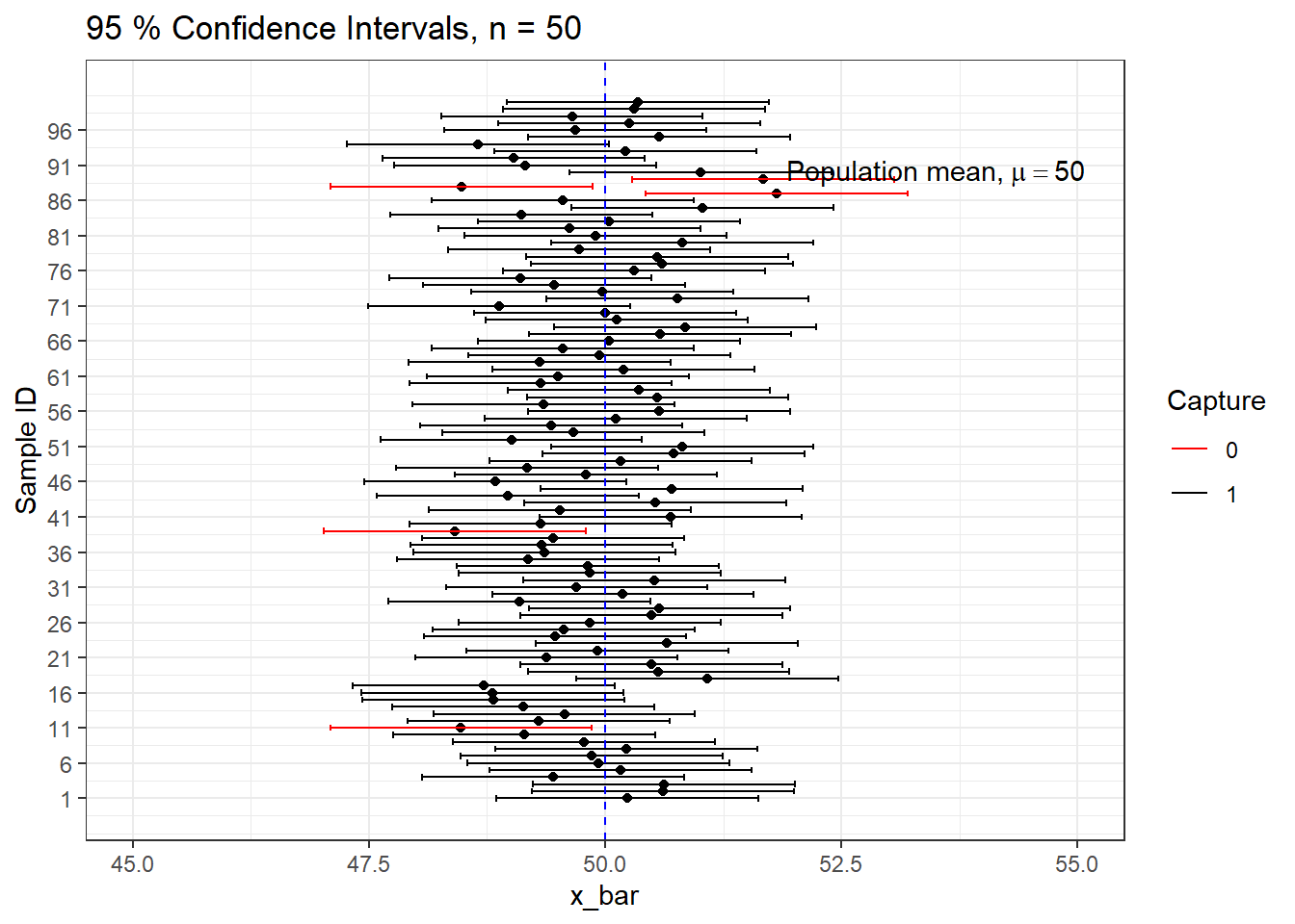
We can see that out of 100 CIs , 95 of them contain true population mean \(\mu=50\) and the rest 5 do not.
| \(1-\alpha\) | \(\alpha\) | \(z_{\alpha/2}\) |
|---|---|---|
| 0.90 | 0.10 | 1.645 |
| 0.95 | 0.05 | 1.96 |
| 0.98 | 0.02 | 2.33 |
| 0.99 | 0.01 | 2.575 |
10.2.4 Interval estimate of a population mean: \(\sigma\) unknown
The \((1-\alpha)100\%\) confidence interval for \(\mu\) is :
\[ \bar x \pm t_{\alpha/2} \frac{s}{\sqrt n} \tag{10.2}\]
Or,
\[ \bar x-t_{\alpha/2}\frac {s}{\sqrt n}, \bar x+t_{\alpha/2}\frac {s}{\sqrt n} \]
We can express this confidence interval in a probabilistic way:
\[ P\left( \bar x-t_{\alpha/2}\frac{s}{\sqrt n}<\mu<\bar x+t_{\alpha/2}\frac{s}{\sqrt n} \right)=1-\alpha \]
Here, \(t_{\alpha/2}\) is the \(t\) value providing an area of \(\alpha/2\) in the upper tail of the \(t\) distribution with \((n-1)\) degrees of freedom that is \(P(T>t_{\alpha/2,n-1})=\alpha/2\).
Problem 9.5 (Keller 2014, 341) In a survey conducted to determine, among other things, the cost of vacations, 64 individuals were randomly sampled. Each person was asked to compute the cost of her or his most recent vacation and the sample mean was $1810.16. Assuming that the standard deviation is $400, estimate with 95% confidence interval for the average cost of all vacations.
Solution: Let, \(X\) be the vacation cost in $. Also let \(\mu\) be the mean of all vacations.
Here sample size is, \(n=64\) with the sample mean , \(\bar x =\$ 1810.16\).
The assumed (population) standard deviation, \(\sigma=\$400\). Since the sample size is sufficiently large so according to CLT, \(\bar X\sim N(\mu, \sigma_{\bar X}^2) \ \ approximately\) .
Where \(\sigma_{\bar X}=\frac{\sigma}{\sqrt n}=\frac{400}{\sqrt 64}=50\)
For 99% confidence interval (CI), \(z_{\alpha/2}=2.575\).
So the 99% CI for the \(\mu\) is:
\[ \bar{x} \pm z_{\alpha/2} \times \frac{\sigma}{\sqrt{n}} \]
\[ Or,1810.16 \pm 2.575 \times 50 \] \[ Or, 1810.16 \pm 128.75 \]
\[ [1681.41, 1938.91] \]
\(\therefore P(1681.41<\mu<1938.91)=99\%\).
Problem 9.6 (Keller 2014, 340) It is known that the amount of time needed to change the oil on a car is normally distributed with a standard deviation of 5 minutes. The amount of time to complete a random sample of 10 oil changes was recorded and listed here. Compute the 99% confidence interval estimate of the mean of the population.
11, 10, 16, 15 ,18, 12 ,25,20, 18 ,24
Problem 9.7 (Newbold, Carlson, and Thorne 2013, 302) How much do students pay, on the average, for textbooks during the first semester of college? From a random sample of 400 students the mean cost was found to be $357.75, and the sample standard deviation was $37.89. Assuming that the population is normally distributed, find the 95% confidence interval for the population mean.
Problem 9.8 (Newbold, Carlson, and Thorne 2013, 302)Twenty people in one large metropolitan area were asked to record the time (in minutes) that it takes them to drive to work. These times were as follows:
30, 42, 35, 40, 45, 22, 32, 15, 41, 45, 28, 32, 45, 27, 47, 50, 30, 25, 46, 25
Assuming that the population is normally distributed find the 99% confidence interval for the population mean of time it takes to drive to work.
10.2.5 Interval estimation for a population proportion : Large sample
From previous chapter we know if \(np\) and \(np(1-p)\) is equal or greater than \(5\) then the sample proportion \(\hat p\) will approximately follow normal distribution with mean \(p\) and variance \(\frac{p(1-p)}{n}\).
Mathematically,
\[ Z=\frac{\hat p-p}{\sqrt {\frac{p(1-p)}{n}}}\approx follows \ \ N(0,1) \]
Since \(p\) is unknown we estimate \(var(\hat p)\) as \(\frac{\hat p(1-\hat p)}{n}\).
Confidence Interval for Population Proportion, \(p\) (Large Samples)
\[
\hat p\pm z_{\alpha/2} \sqrt {\frac{\hat p(1-\hat p)}{n}}
\tag{10.3}\]
which is valid provided that \(n\hat p\) and \(n(1 - \hat p)\) are greater than 5.
Problem 9.9 (Newbold, Carlson, and Thorne 2013, 305) In a random sample of 95 manufacturing firms, 67 indicated that their company attained ISO certification within the last two years. Find a 99% confidence interval for the population proportion of companies that have been certified within the last 2 years.
Problem 9.10 (Newbold, Carlson, and Thorne 2013, 305) From a random sample of 400 registered voters in one city, 320 indicated that they would vote in favor of a proposed policy in an upcoming election. Find a 98% confidence interval for the population proportion in favor of this policy.
10.3 Sample size determination: Large Population
10.3.1 Sample Size for Population Mean
If \(E\) be the margin of error (E), \(\sigma\) be the population standard deviation (assume known) then the required sample size (n) to estimate a population mean \(\mu\) with \((1-\alpha)\times 100\%\) confidence level is:
\[ n=\left( \frac{z_{\alpha/2} \sigma}{E} \right)^2 \tag{10.4}\]
Sample size determination: Derivation
From the interval estimation regarding \(\mu\) we know
\[ P(\bar x-z_{\alpha/2} \frac{\sigma}{\sqrt n}<\mu<\bar x+z_{\alpha/2} \frac{\sigma}{\sqrt n})=1-\alpha \]
That is,
\[ P(\bar x-E<\mu<\bar x+E)=1-\alpha \]
Hence we can write,
\[ E=z_{\alpha/2} \frac{\sigma}{\sqrt n} \]
Solving for \(n\) we have
\[ n=\left( \frac{z_{\alpha/2} * \sigma}{E} \right)^2 \]
Problem 9.11 (Keller 2014)
a) Determine the sample size required to estimate a population mean to within 10 units given that the population standard deviation is 50. A confidence level of 90% is judged to be appropriate.
b) Repeat part (a) changing the standard deviation to 100.
c) Re-do part (a) using a 95% confidence level.
d) Repeat part (a) wherein we wish to estimate the population mean to within 20 units.
Problem 9.12 (Keller 2014) The operations manager of a large production plant would like to estimate the average amount of time workers take to assemble a new electronic component. After observing a number of workers assembling similar devices, she guesses that the standard deviation is 6 minutes. How large a sample of workers should she take if she wishes to estimate the mean assembly time to within 20 seconds? Assume that the confidence level is to be 99%.
10.3.2 Sample Size for Population Proportion
If \(E\) be the margin of error (E), \(p*\) be the assumed population proportion or planning value of \(\hat p\). Then the required sample size (n) to estimate a population proportion \(p\) with \((1-\alpha)\times 100\%\) confidence level is:
\[ n=\frac{z_{\alpha/2}^2\times p^* (1-p^*)}{E^2} \tag{10.5}\]
N.B: From Equation 10.5 it can be proved that the sample size will be maximum for \(p^*=0.5\). So to obtain the maximum sample size we can take \(p^* (1-p^*)=0.5\times 0.5=0.25\) in Equation 10.5.
Problem 9.13 (Anderson 2020) At 95% confidence, how large a sample should be taken to obtain a margin of error of 0.03 for the estimation of a population proportion? Assume that past data are not available for developing a planning value for population proportion \(p\) ?
Problem 9.14 (Anderson 2020) Stay-at-Home Parenting. In June 2014, Pew Research reported that in 16% of all homes with a stay-at-home parent, the father is the stay-at-home parent. An independent research firm has been charged with conducting a sample survey to obtain more current information.
a. What sample size is needed if the research firm’s goal is to estimate the current proportion of homes with a stay-at-home parent in which the father is the stay-at-home parent with a margin of error of 0.03? Use a 95% confidence level.
b. Repeat part (a) using a 99% confidence level.